
So, we talked about how we can use neural networks to build a face recognition system. Then we talked about word embeddings, a method for representing textual data. In this article, we are going to talk about all the steps in a typical machine learning project, from start to finish. Are you ready? “Yeah!”—you shout. Let’s go!
Step 1: Data Acquisition
As we said countless times, for any ML problem we need... DATA. Where can we find data? If we are lucky, our client will provide us with a working dataset that we can experiment with. If not, then we have our friend—the internet.
There are a lot of publicly available data repositories that we can access. We have benchmark datasets that scientists use to evaluate their research. We also have competition datasets that ML enthusiasts use to showcase their ML skills.
After acquiring the appropriate dataset, in some cases even multiples of them, we go to our next step—data wrangling.
Step 2.1: Data Wrangling
The datasets we acquired most likely didn’t come in the format we wanted, so we need to adapt them. This is data wrangling: we consolidate, we clean, we transform. We also evaluate the usability of our data. Data wrangling takes most of our time, between 50% and 80%, so learn to like it. This process is extremely ad-hoc with little to no standardization. But that’s the beauty of it. We experiment to get what we want.
“What problems do we expect to face?”—you ask. Missing data, incorrect data, and inconsistent data. Here, we often need expert intervention. Crowdsourcing platforms will also do. “How do we diagnose problems?”—you wonder. The easiest way is with simple stats and visualization. But, be careful to choose the appropriate plots. This problem is increasingly more difficult as data gets larger. So, sampling strategies to the rescue!
“What is sampling though?”—you wonder. Sampling is acquiring a portion of the data that represents it well. There are a ton of sampling strategies: we can sample uniform at random, we can sample such that the class distribution is preserved, we can sample based on importance, and so on and so forth.
Step 2.2: Data Preparation
With ML models, it usually holds: “garbage in, garbage out.” We need to prepare our data for whatever follows. We need to handle the uncertainty that can arise from measurement errors, chosen sampling strategies, etc. We need to execute feature engineering—a form of “dark art” that was, fortunately, mitigated by deep learning. We need to detect relevant features, either offline or online. This will help our model perform better. We need to normalize features (by using logarithmic scaling, min-max scaling, or standardization). This will improve the learning process. Some models require that our features be discretized. In some cases, we need to completely transform our data to get meaningful samples for our specific problem. Remember word embeddings? These high-dimensional vectors are really neat. However, beware of the curse of dimensionality.
After producing a big fat dataset to work with, we analyze.
Step 3: Data Analysis
How do we get acquainted with our data? Once more, we can visualize data. To detect the distribution of each feature, we use histograms. To check the correlation between features, we use scatter plots. Box plots reveal outliers. QQ plots compare distributions.
There are different types of data distributions: Poison—number of visits to a given website in a fixed time interval, Exponential—the interval between two such events, Binomial—number of heads in 10 successive coin flips, etc. Data can be skewed—20% of the world's population receives 80% of the world's income, right? Power law, a right-tailed distribution, is linear on a log-log plot. Special care needs to be taken with skewed data.
High-dimensional data can’t simply be visualized. So we can use projection techniques like PCA or t-SNE to bring the data in low dimensions.
What else can we use? We can use descriptive statistics: mean —to get the average value, variance—to get the spread, min, max, median, quartiles, you name it. For skewed distribution, the mean is meaningless. So is the variance. We use the median instead. Some descriptive statistics are robust to outliers, like median and quartiles, and some are not, like mean and variance.
We can detect the distribution with statistics: Kolmogorov-Smirnoff test. We can check correlation with statistics: Pearson correlation coefficient for linear dependency, Spearman’s rank correlation coefficient for monotonic dependency, Kendall rank correlation coefficient for the ordinal association. Correlation is tricky. High chicken consumption doesn’t cause an increase in crude oil imports in the US!
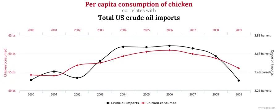
Image courtesy: https://www.tylervigen.com/spurious-correlations
Remember, whenever you report statistics you need to quantify how certain you are. Confidence can be reported by using bootstrap resampling—sample with repetition and measure multiple times, then use the values to calculate the confidence interval. Also, be aware of aggregates. Trends can appear in different groups but disappear when groups are combined—the Simpson’s paradox. And the pinnacle of all: hypothesis testing and the infamous p-value used to draw conclusions about a population parameter or a population probability distribution.
Step 4: Big Data
How much data do we need, that’s the question? As much as we can get, that’s the answer. However, with lots of data, we introduce a problem: it simply cannot fit in our computer. Even less so in the memory of our computer. What do we do? We distribute! We set up a cluster of computers to process our data. Or, if we are lazy and don’t want to bother with maintenance, scaling, fault-tolerance, virtualization, etc. we make Jeff Bezos a tad richer by using AWS. Now, how do we program these beasts? DIVIDE AND CONQUER to the rescue. We use a well-known analytics engine, like Spark, to handle our data well.
Now, we’ve handled our data well and it’s time for the cool part. Brace yourselves, ‘cause we are about to do some magic!
Step 5: Model Selection
How do we choose the class of models for our task? It’s super easy! Do we have to predict a continuous label, like a house price? We choose a regressive model. Do we have to predict a categorical label, like if an email is a spam or not? We choose a classification model. Whoops! we don’t even have a label to predict? Not to worry! We can detect structure in the data, like clusters of users in our web store so we can bombard them with personalized marketing campaigns.
How do we know which model to choose? Well, we don’t. What we do instead is choose the simplest model we can think of. This will set our baseline of how well we perform. Then we try to improve this performance by extending the simple model or by using a more complex model. Here is a piece of advice (for free!):
Always start simple.
Of course, there are other criteria for choosing a model: predictive performance, speed, scalability, robustness, interpretability, compactness, etc.
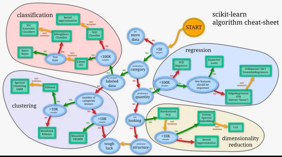
Image courtesy: https://scikit-learn.org
We’ve decided on which model to use. Now what? Now we train our model.
Step 6.1: Model Training
Our model has parameters that we need to set so it can do its job. How do we do that? We minimize a loss function—how far is the model’s prediction from the label, on average, by changing the parameters. Depending on the class of models, we can use the mean squared error, for regressive models, and cross-entropy, for classification models. For clustering... it’s a bit more complicated.
How do we minimize the loss function? Let’s jump to our ML kitchen. Remember the dataset we so carefully prepared? We take it and slice it into two parts: one for training and one for testing, or 70%/30% of the original dataset. Even better. We slice it into three parts: one for training, one for evaluation, and one for testing, or 60%/20%/20% of the original dataset. We need to be sure that the slices are non-overlapping. We also need to be sure that each slice preserves the class distribution.
Let’s move the last two slices aside. We are left with our training slice. Boy, I’m getting hungry and so does our model.
We set our model in a training state (in the train state, the model’s parameters are updated). We start feeding our model samples, or batches of samples right before it starts learning everything by heart. This is necessary because we want our model to perform well on unseen samples or, as we ML engineers like to say, we would like the model to generalize well. “How do we know if it generalizes well?”—you ask.
We take the testing slice. Right after we’ve fed the model with the whole training slice, we put the model in an evaluation state (in the evaluation state, the model’s parameters are not updated). Then we feed the model with the training slice and calculate an evaluation metric, like the accuracy. Remember skewed data? Well, accuracy doesn’t work. So use the F1 score — the harmonic mean of precision and recall, calculated by using the not so confusing confusion matrix.
We repeat these two steps as long as the metric improves. But something strange happens. At one point, this metric starts to worsen. We stop! It is at this point that our model is trained sufficiently.
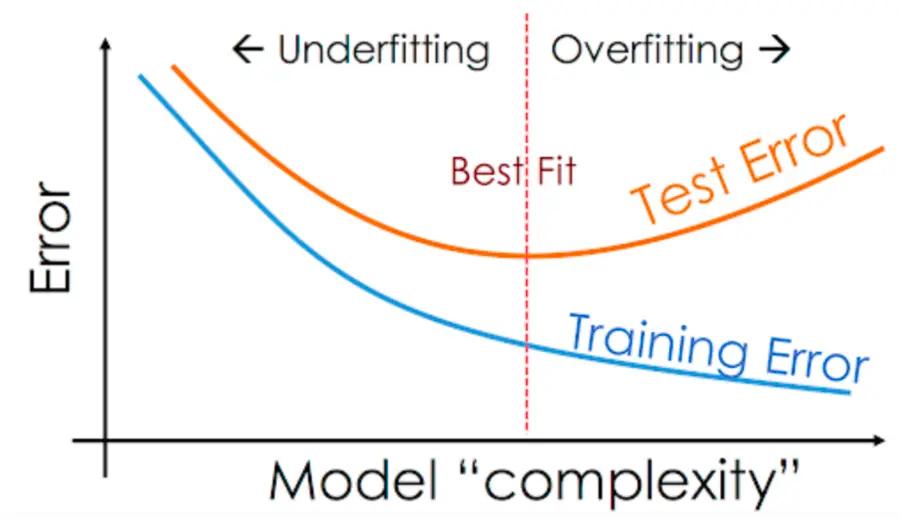
Complex models tend to overfit. We fight this with regularization—we penalize large parameters more. Simple models tend to underfit. We fight this by using more complex models. Complex models tend to overfit—RECURSION DEPTH EXCEEDED.
This is all part of the infamous bias vs. variance dilemma.
“What about the evaluation slice?”—you wonder. Good point!
Step 6.2: Hyperparameter tuning
Besides the parameters, each model has hyperparameters that need to be set, unfortunately, by hand. Luckily, there are not as many. Let’s take neural networks for example. Some of its hyperparameters are: number of hidden layers, number of neurons per layer, weight initialization, activation function, dropout, learning rate, momentum, number of epochs, batch size, etc.
How do we proceed? We choose one combination of hyperparameters, execute Step 5, but instead of using the test slice, we use the evaluation slice for calculating the evaluation metric. We repeat until all the possible combinations for our hyperparameters have been exhausted. We choose the one combination with the best performance on the evaluation slice. Finally, we report the evaluation metric on the test slice.
An honorable mention is k-fold cross-validation. It’s a more advanced technique where we slice the dataset k times. We train using the first k-1 slices and evaluate using the last slice. We repeat this in a circular fashion. The average accuracy tells us how well our model performs.
That’s it. Now we are ready to use our model in the wild.
Step 7: Deployment
We’ve come to the last piece of our puzzle, the model deployment. In recent years we learned that the need for reliable and efficient deployment of models in production was a necessity not a commodity. Because of this, we’ve developed a whole new field in IT, called MLOps (ML + DevOps). Once developed in isolated environments, Machine Learning Engineers, Data Engineers, and DevOps Engineers work together to bring the model into production by increasing automation and improving the quality.
I can’t believe we are at the end of our journey. To be frank, we’ve covered a lot of ground and I hope that you appreciate machine learning more. How do you feel buddy? “I am… speechless. I want to hear more! Let’s go back to neural networks...”
About the Author
Mladen Korunoski is a data scientist working at our engineering hub in Skopje.
Mladen's main interests are Machine Learning and Software Development. In software development, Mladen is versed in multiple programming languages and frameworks. In machine learning, most of his experience is in Natural Language Processing (NLP).