
Welcome back to your favorite blog series! In the previous part, we talked about machine learning in the cloud and presented the benefits and drawbacks. Also, we described the problem we are trying to solve: customer satisfaction with airline services. In this blog post, we continue our journey and introduce an AWS service that will be used for cleaning and transforming our training and test data.
AWS Glue DataBrew
Hooray! We are jumping into our first cloud service. AWS Glue DataBrew is a visual data preparation tool that enables both data scientists and analysts to clean and normalize data, without the need to write code. Using DataBrew helps reduce the time it takes to prepare data by up to 80 percent, compared to custom-developed data preparation.
AWS Glue DataBrew offers over 250 ready-made transformations to automate filtering anomalies in data, converting data to standard formats, and correcting invalid values. The service provides a visual interface that allows you to easily connect to data stored in Amazon S3, Amazon Redshift, Amazon RDS, any JDBC-accessible storage, or data indexed in AWS Glue Data Catalog.
Once the data is prepared, it can be used by other AWS services such as Amazon Redshift and Amazon Athena (for analytics), Amazon Quicksight and Tableau (for Business Intelligence), or Amazon SageMaker (for machine learning). In our project, Amazon SageMaker will be used to prepare and train our model, but we’ll leave that for the final part of this blog post series.
Prerequisites for DataBrew
Keep in mind that you need the following steps already set up to get started with AWS Glue DataBrew (hence this project) which are not covered in this blog post.
- You need to register and set up an AWS account
- You should create an S3 bucket. The process is straightforward and can be done in a few simple steps. Just follow the instructions provided by AWS.
- You should create an IAM role with both DataBrew permissions selected, having read accessed your newly created S3 bucket.
So, let’s get started with DataBrew and our data preparation!
Getting started with AWS Glue DataBrew
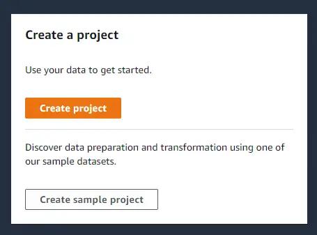
First, look up AWS Glue DataBrew in the Management Console and open it up. On the service landing page, click on the “Create Project” option.
Afterwards, a new configuration window appears where we name our project. Let’s call it “AirplanePassengerSatisfaction”. We also select the option to create a new recipe, which is named automatically based on our project name.
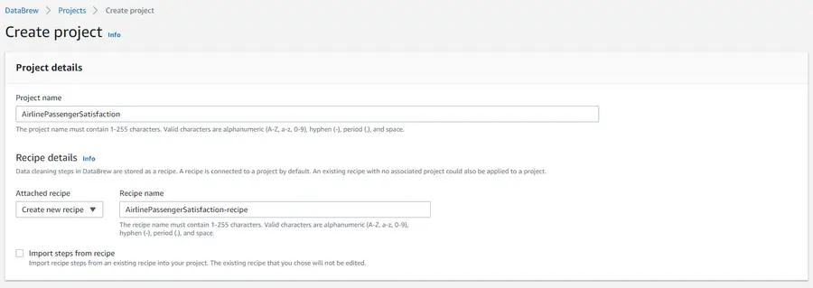
In DataBrew, a recipe is a set of data transformation steps that the user defines for the data in the project. You can apply these steps to a sample of your data, or apply that same recipe to the entire dataset. Using DataBrew, we can visualize the effect of each step in the dataset until we reach the desired final result. We will show an example of a recipe in just a few moments.
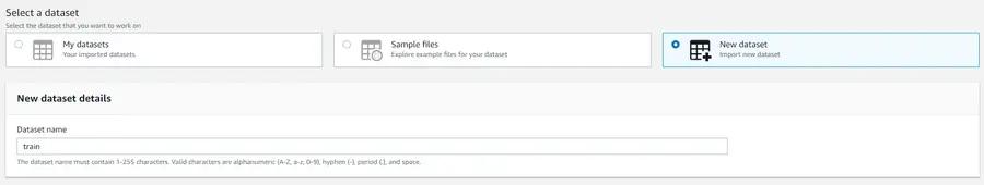
Next, we select our dataset. Since we are uploading our training dataset for the first time, we need to choose the “New dataset” option and name it accordingly. Let’s name it train (so creative right?)
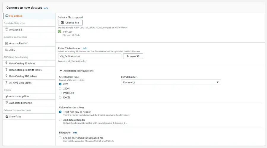
When the “Connect to new dataset” section appears, we simply select our file for upload (train.csv) and choose the S3 bucket to store the file. The rest of the options vary based on the type and content of the file.
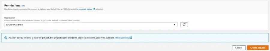
Finally, select the IAM role you’ve created for the project and hit the “Create Project” button.
Once the session is loaded, we’ll immediately see a 500-row sample of our data. For each column, we also get some statistics such as value distributions, median, minimum and maximum values. In order to see some statistics for the full data, we need to run and create a new “Data Profile” which is done in the “Profile” tab. But before we jump into that, we can start preparing our recipe.
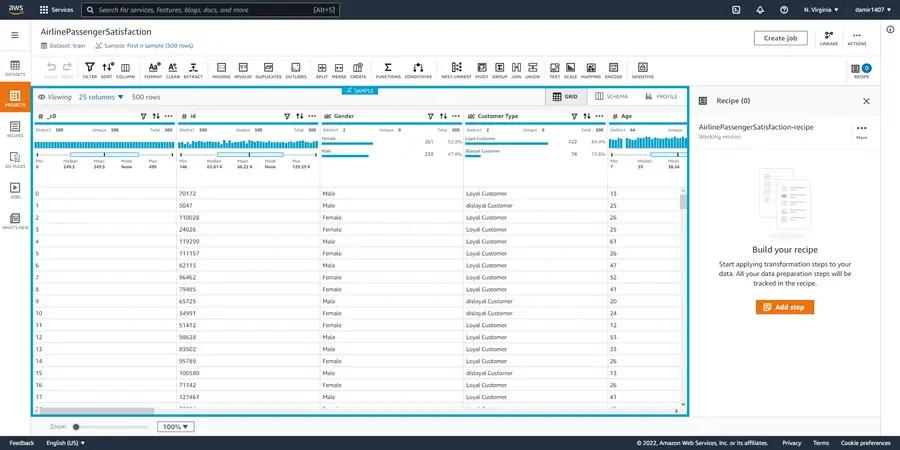
As we investigate the dataset, we can see that it has a total of 25 columns. For this “interim” step, we will perform the required transformations and generate the recipe as follows:
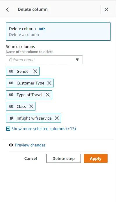
- Delete the uninformative “_c0” and “id” columns
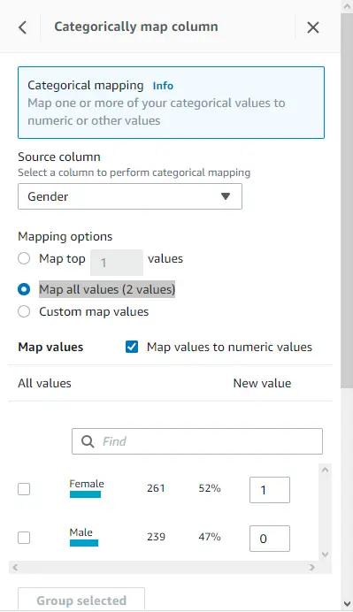
- Encode the binary categorical variables, map them into new columns and delete the original ones.
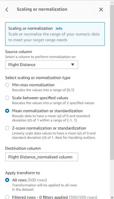
- Normalize the remaining numerical columns with Mean normalization, map them into new columns and delete the old ones.
Note that non-binary categorical variables also need to be one-hot encoded, but before doing that we will create a new job that will produce a new “interim.csv” training dataset with the above mentioned transformations and store it in our S3 bucket. This interim dataset will be imported in the same manner as the raw dataset and be used to generate a new data profile.
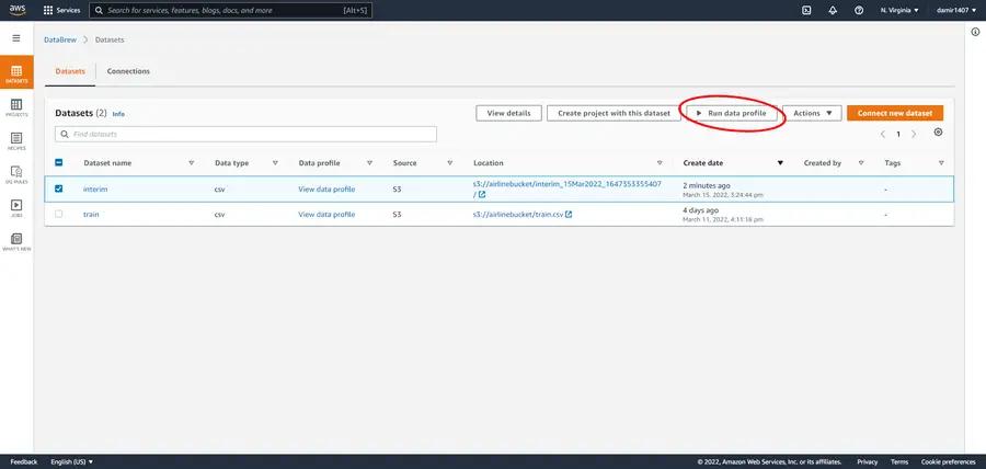
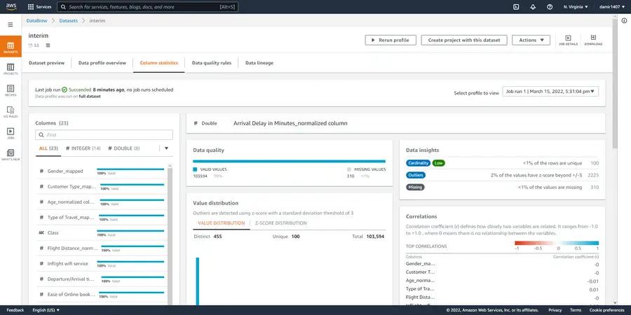
Once our interim training dataset is ready, we can import it and run the data profile job as shown in the image below.
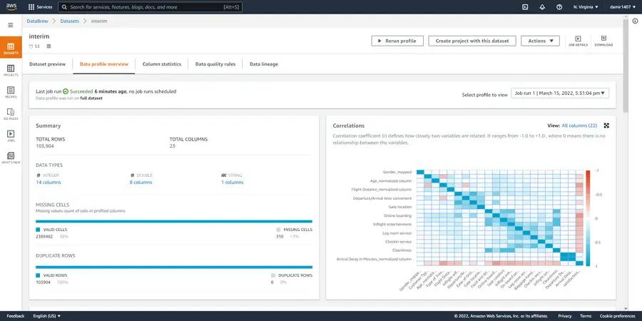
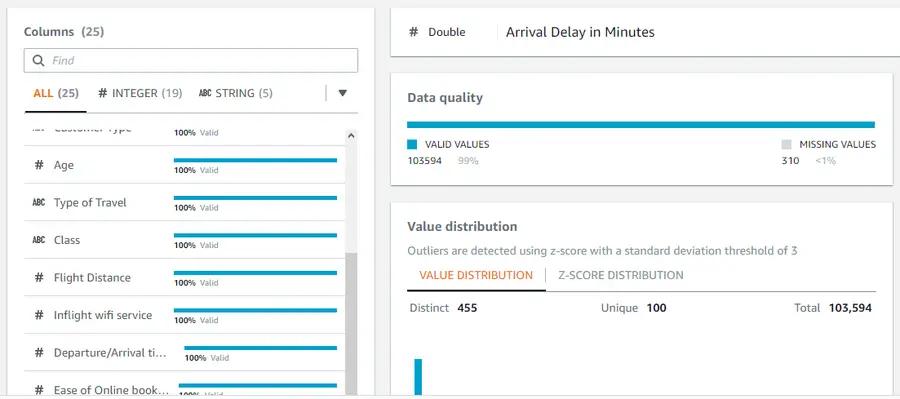
The data profile, and especially the correlation heat map, will help us detect informative variables once we start working with our prediction model. The data profile also provided us with additional information. We can see that there are some missing values in our dataset (around 300 of them), but without any duplicates. If we switch to “Column statistics”, we can see exactly which column is missing data. In our case, all the missing values are from the “Arrive Delay in Minutes” column. So, we should definitely fill those in our recipe! Additionally, on this page you can see statistics of the full dataset for each column.
Column statistics
So, we need to make the following additions to our recipe:
- Fill in missing values in the “Arrive Delay in Minutes” column.
- One-hot encode non-binary categorical variables, map them into new columns and delete the original ones.
Luckily, DataBrew allows us to use versioning on our recipes, so we can keep track of our changes.
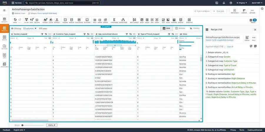
Once we have added the remaining steps in the recipe, our workspace should look like the image below.
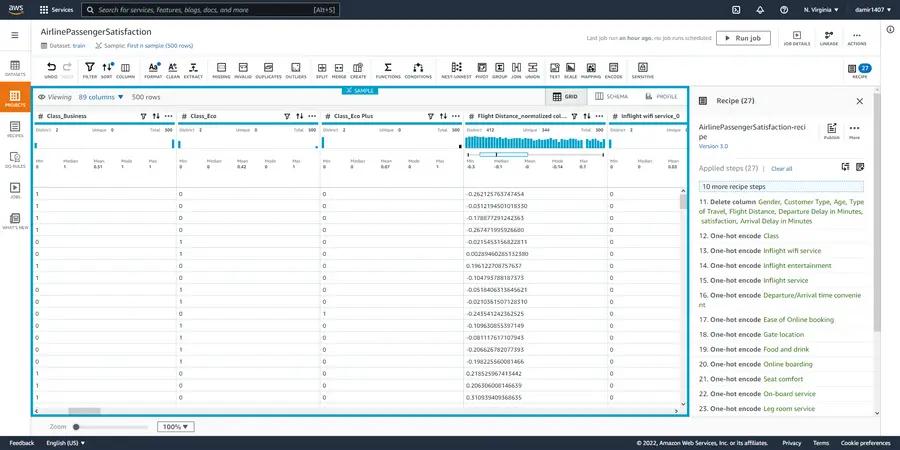
Similarly as before, we should create a new job called “processed”, link it to our existing project and run that job. That will create our final processed training dataset to be used in our next blog posts!
Thank you for your attention, that’s all for Part 2 of our blog series. In the next one, we will learn how to set up CI/CD pipelines in order to automate the release process of our recipes using AWS CodePipeline, AWS CodeCommit and AWS Lambda.
About the author
Damir Varesanovic is a Software Engineer working at our engineering hub in Bosnia and Herzegovina.
Damir’s areas of expertise are Data Science and Software Engineering. He is proficient in Python, and he has deep knowledge of algorithms, SQL, and applied statistics. He is also experienced in the area of backend frameworks, such as Spring, Android, .NET, Django, Flask, and Node.js, and he used them in various projects during his professional career.
-1.png&w=3840&q=50)
-1.png&w=3840&q=50)
